Category Archives: Articles

Article-length features written by Jim Johnson

Seven Habits of a Highly Effective Astrophotographer

There’s just one thing that I don’t want to learn, and that’s a lesson.
– Homer J. Simpson.

Generally, I find that as I make astronomy easier, I tend to do more of it. This note is about the lessons-learned that I have applied to make astronomy easier, and then do more of it.

MAINTAIN A WARM SCOPE

As my setup is quite sophisticated, setup and tear down time for every observing session can be as much as two hours. By having a telescope on a mount with decent polar alignment shortens the time to about twenty minutes to uncover the scope, add a camera, and add power. There have been occasions that I have unexpectedly woken up in the wee hours of the morning, found clear skies, and decided to go out to the scope, and add a camera and power for an imaging session. I seriously doubt that I would ever do a from-scratch setup in the middle of the night. Two keys to making this possible are a 365-day cover, and a couple of pavers set into the turf to prevent the telsecope legs from sinking into the soft soil.

IMAGE REMOTELY

Sitting alone in the dark to manage an imaging session is not fun. Doing it on a freezing cold night is even less fun. Being able to spend 15 minutes to prepare for a session during the daylight, and another 15 minutes to polar align and get an initial focus position removes a lot of imaging downside. Being able to conduct an imaging session from a warm house after polar aligning and focusing is fun. The two keys to making this possible are having an extra computer so that I can leave one connected to accessories at the scope, and another computer that can remotely access the scope-side computer from in the house or camper. The other key is a nano router that enables remote access when away from the home WIFI network.

BUNDLE WIRES

I use many accessories to automate various aspects of my imaging sessions, which include mount controller, electronic focuser, guide camera, filter wheel, and main camera. These accessores require 12vdc power or data (USB) connections, or both. My single cable consists of about ten individual wires. In the bundling. At some point in the development of my setup, the wires hanging off of the back of my scope made it look like a ghilley suit, and I had a rat’s nest of wires beneath the tripod. Slewing was hazardous because wires were dragging behind the scope, and prone to snag. My solution was to bundle wires so that a single cable runs from the scope, connects to the mount controller, and then to a power board on the ground. I leave connection ends where they need to be to connect to their device. Running each of these wires separately, and then zip tying them to prevent snags takes a considerable amount of time and effort. With my present setup, I pick up one cable (instead of ten wires) I spend about a minute making wiring connections, and I need to add only one zip tie.

WRITE

This item goes to the Jim-ism, you won’t remember as much as you think that you will.

Write and use workflow documents. Common mistakes that I make during an imaging session are forgetting to do something important, doing it in the wrong sequence, or just plain doing it wrong. This goes to the Jim-ism, you won’t remember as much as you think that you will. I add the word “use” to the title of this section, because I notice several instances of making rookie mistakes by going off script. In addition to keeping me on track, a write work flow is a great place to insert an obscure new step that I learn, and might be otherwise likely to forget by the time of my next imaging session. For me, it is so tempting to just forge ahead on my own, but looking at a script keeps me on track. In places were I know the procedure very well, I might read (glance at) several steps, execute them, then read again to make sure that I covered everything. I tend to pare down the steps as I become more proficient. I no longer need the details, so polar alignment, for instance, has become a single step. I consider my workflow documents to be as important as my equipment and my skills. I do better astronomy and have fewer imaging sessions end badly when I stay on script.

Write up observing reports. By writing observing reports, I have a record of what I have done, and useful patterns emerge. I also document the problems that I had, so that I can track them to resolution. Just the act of writing them alone forces me to think more deeply about what I have done during a session. I can also just look at the titles and see overarching patterns, like how many sessions have been dedicated to one kind of astrophotography or another, or how long it has been since I have devoted a session to a certain kind of session.

DRESS FOR THE WEATHER

Even if I have the gear, I must be sure to wear it when appropriate. I have had imaging sessions ended by cold weather because I tried to tough it out early on, and then found that I couldn’t wam up after having let myself get cold. I have heard it said that the best way to stay warm is to never let yourself get cold. My warm weather gear consists of a warm hat, a parka under which I wear several layers, ski pants under which I wear several layers, insulated boots in which I can put battery powered feet wamers, and thin and thick gloves in which I can put chemical hand warmers.

GO TO DARK SITES

DSO imaging at a dark site is more efficient than at a bright sky site. For DSO imaging in my backyard under a Bortle Class 6 sky, eight to ten hours of image data collect is required to support a high quality image of a dim nebula. At a dark site, two to four hours of collection is sufficient for many dim targets. As my DSO imaging skill improves, I expect to collect on multiple targets in a single night at a dark site.

DAILY SCAN AND PLAN

It is my habit to do a scan soon after I am awake every morning. I conduct this scan with an eye toward what astronomy things that I want to do on that day. First, I want to know what my commitments are. That can take out small or large parts of day, take out a whole day, or take out several days. Before deciding on the day’s activities, I make a weather and conditions-based decision about what imaging that I might want to do. For example, if the moon is out, I might image it, planets, or star clusters. If the moon is away, I might choose nebulous targets. The seeing and transparency forecast might affect my decision. After deciding that, I consider what daytime work might be needed to support that evening’s imaging. I also consider other equipment work or tweaks that I can accomplish.

Do daytime work during daylight hours. I am constantly alert for opportunities to accomplish every task that I can during daylight hours. First of all, any task is likely to be easier in the daylight, so why not do then what can be done then? Secondly, clear night skies are a rare commodity, so why defer tasks more appropriate for daylight hours until darkness?

Make the best use possible of marginal nights. One of my chief goals is to be as prepared as possible for collecting the highest-quality image data on nights with the best transparency, in the darkest sites. If I defer testing and tweaking of equipment, for instance, to these nights, then I have squandered premium image time on something that very well could have already been done. For instance, if I can tune my autoguiding on marginal nights, then I am prepared to collect image data when a rare premium night comes along. Other tasks are even more obvious. I would never attempt a delicate backlash adjustment at night.

Practice. This section goes to another Jim-ism, one must learn new things quicker than onld ones are forgotten in order to improve one’s skill. All aspects of a session need to be practiced. If I set up during an afternoon that promises marginal skies that evening, and then it is completely clouded out, then I have paracticed setting up. If I work with my autoguiding system on a marginal night, then I have practiced imaging. If I have spent most of the summer and the entire fall on planetary imaging, then I have not practiced DSO imaging, and it will take me a while to get good at it again.

Dewy or Don’t We?

I have been so drawn to this title that has been floating around in my head that I just had to start writing about it. You may find the idea of anything floating around in my head sufficiently amusing that there is no need for you to read any further.

Dew season is coming up, so we may as well get ready for it. I have done some reading on dew, but I am not yet at the expert level. My aim in writing on this topic is help me clarify my thoughts, and to help raise awareness and stimulate thought in a manner that will help astronomers meet, understand, and defeat dew.

The dew point is one of the keys to understanding dew. The atmosphere always contains moisture, sometimes more of it than others. As the temperature drops from daytime into nighttime, the atmosphere is able to hold less moisture than when it is warmer. The dew point is a function of the amount of moisture in the atmosphere, and temperature. This function yields a temperature at which the atmosphere is “forced” to begin releasing moisture as water droplets.

But this is not the final answer. Astronomers must deal with the “chilling effect” of the night sky (that we are out to observe) on their equipment. Dew does not “fall” onto the upper surfaces of our equipment, it forms there as a result of the chilling effect. Our equipment radiates heat (IR radiation) in all directions. The bottoms and sides of our equipment gets some heat back in the form of radiation from our surroundings. The clear air above us, however, does not give back nearly as much heat as our surroundings on the the ground. This causes the upper surfaces to chill faster, which in turn hastens the formation of moisture on these surfaces.

How can the weather forecast help us? I don’t know exactly, but here is a possibility. I have observed for sometime that the forecast usually predicts that during the daytime the air temperature will be well above the dew point. On most nights, and for most of the night, the temperature and dew point are about the same. Perhaps when the air temperature falls to the dew point (and probably a few degrees above that point) is when dew protection is needed. In the future, I intend to note the time in the forecast at which the air temperature drops to the dew point, and observe when dew actually starts forming. If I am in the back yard, next to my weather station (Google: Weatherunderground KMDASHTO6), it is easy to monitor conditions.

Here is another exploitable fact: both glass and painted surfaces radiate heat very well, and are both prone to collecting condensation. Using painted metal surfaces as a proxy for glass, even if we have protection in place on the glass, we can gain a sense of when and under what conditions dew forms.

A dew shield is the first line of defense against dew forming on our optics. When a telescope is not pointed straight up, dew shields give us some protection from dew. Not because they prevent the dew from falling onto the glass, but because they are a barrier between the forward facing optics and the chilling effect of the night sky above. Shields do not help much when observing near the zenith.

A slight breeze can be helpful. This is not because of a “drying” effect of the breeze, but because air that is kept slightly warmer by radiation received from our surroundings is moving over the optics. A dew shield, counterintuitively, might prevent the breeze from “warming” our optics and could actually increase the likelihood that dew will form.

The next line of defense is applied heat. It doesn’t take much heat. The optics that we are trying to protect need be only slightly warmer than the surrounding air, and not necessarily warm to the touch. Three ways to warm optics come to mind. Dew heaters, usually as strap connected to a controller that controls the amount of heat applied (and the drain on valuable and heavy battery capacity) are convenient. Probably best monitor the ambient temperature relative to the dew point and begin applying heat before the dew ever forms to avoid it all together. Otherwise one might end up waiting some period of time for optics to clear after the dew has formed. 12v hair dryer type devices are used by some astronomers, but periodic reapplication of heat is required. I have heard of astronomers using rubber bands to affix chemical hand warmers to Telrads. 

Here is an experiential data point: I turned on an Astrozap dew heater strap and controller on my 4″ refractor AFTER dew had begun to form on the objective lens at the during a photography session on October 14th. It took about 15 minutes with the power setting at full/high for the dew to clear. I turned it down to about 30% and the lens stayed clear for the remainder of the session. In the future, I plan to turn on the dew heater earlier (guided by forecast and/or actual conditions), and experiment with even lower settings. Perhaps there is some factor that I can consider that will suggest whether a lower or higher setting is appropriate.

There are many finer points to shielding and heating solutions, but I think that this a good start with regard to understanding and solving the dew problem. I think that the key to being more effective in combating dew is to be observant of forecasts, weather conditions in real time when possible vs. when dew actually forms on our equipment. Also, gaining experience with how much heat to apply (or how much of an amperage load to allow on our batteries) to keep dew from forming will be helpful as well.

© James R. Johnson, 2021.
jim@jrjohnson.net

Portable Power Solutions for Astronomers: Part 5, Conclusion

We have reached the end of a three-part series of articles on the power required to get an astronomer through a night of observing. We began by discussing battery types, distinguishing between a battery as but one component of a complete astronomy power solution, and then we identified the other components of this complete solution, which includes a case, outlets and their circuit protection, and a battery charger that will ensure that the battery is ready whenever it might be needed next.

At a high level, we found that battery usage can be defined in terms of a three-way trade space of battery capacity in amp hours, total amp load of the devices drawing power from the battery, and time that the device load can be sustained before the battery capacity is depleted. How the capacity and load relate to time is important because this is the basis for how the adequacy of a battery for a night of astronomy is assessed.

Next, we gave a similar treatment to replenishing the battery’s charge after a night’s use. We found a similar three-way trade space between capacity in amp hours, amperage supplied by the charger, and time. We distinguished between a straight battery charger and a smart charger and identified the advantages of a smart charger when it comes to preserving a battery’s useful life. And finally, we discussed the context for determining the adequacy of a charger, especially when there is limited time to recharge a battery for use on two consecutive nights.

And finally, we discussed some particulars regarding commercially available power solutions, and DIY power solutions. The DIY solutions require much more forethought to ensure that the end product produces the desired result, and we pointed out that some electrical skills and a sense of adventure on the part of the astronomer are required for going this route. But a big advantage that DIY solutions have over commercially available solutions, especially those involving higher battery capacities, is that the DIY solutions can be far less expensive for those who can do it.

We hoped that you have found this series informative, and useful as guide to the research that you may want to do in determining the amount of battery capacity is needed in your power solution, and in determining the correct charging capacity for your needs. And lastly, we hope that you have an appreciation for how commercially available units are alike, how they differ from DIY solutions, and for which might be the better route for you.

We would love to hear about your power solution, how you use it, and how it was decided. Helpful comments below are always appreciated.

© 2021 Jim Johnson and Doug Biernacki

Portable Power Solutions for Astronomers: Part 4, Other Considerations

Upon arriving in the field with a suite of astronomy gear that must be set up before nightfall, an astronomer has a lot of work to do, often in a short amount of time. The considerations discussed in this section are an essential part of how an astronomer gets the job done on time and how the job gets done correctly. These considerations apply to all the astronomer’s equipment, batteries included. And finally, as no battery lasts forever, we will close out this series of articles by discussing factors that can limit a battery’s useful life.

Before going into details, description of commonly encountered power solutions is in order. I use the term “solution” to avoid the names that commercial producers use for their battery equipment (like pack, tank, etc.), and because the specific power equipment that an astronomer selects specifically solves the astronomer’s power problem.

As discussed in Part 1, a complete power solution consists of battery itself, possibly a battery enclosure, possibly a monitoring device or devices, circuit protection for the outlet connections, the outlet connections and a battery charger. The battery is likely to be withing the enclosure, and all the other components are likely to affixed to the enclosure by means of a panel mount. The battery charger restores the battery’s charger, in a manner that preserves the battery’s useful life, and quickly enough that the battery is available the next time that it is needed.

As for the battery itself, all that was said about volts, amps, amp hours and charging in Parts 2 and 3 apply. A monitoring device is required to detect when the battery has reached is maximum safe discharge level so that the battery can be disconnected and not be damaged by being overly depleted. Sometimes a color-coded charger indicator serves this purpose. Circuit protection can be either a circuit breaker or a fuse that interrupts the circuit if a higher load than is anticipated is encountered, usually one for every outlet connector. The most common outlet connector accepts the cigarette lighter plug, but Anderson Powerpole connectors are becoming more common. The enclosure that contains the battery, and to which the other components are mounted, can take a wide variety of forms. Manufacturers’ enclosures are custom made. Trolling motor or other battery boxes are sometimes used by do-it-yourself (DIY) builders of power solutions.

There are four important considerations concerning battery use in the field: handling, setup, connecting, and use. The less time spent on placing the battery into service, the better, because there are so many other details to which the astronomer must attend before darkness arrives.

From a handling perspective, batteries are heavy and can be difficult to transport and handle in the field. Generally, the higher the capacity in amp hours, the heavier the battery. A carrying handle of some type is essential here, as it can allow many batteries to be carried with one hand, leaving the other hand open to carry some other gear. Commercially marketed solutions have handles or carrying straps. Most battery boxes that DIYers use have handles.

Having all of the components mounted on the enclosure helps not only by eliminating setup time, it also prevents polarity errors in connecting components and it prevents components from being forgotten or lost.

Getting polarity correct when connecting equipment is essential and should not be presumed to be as easy as it looks. If a connection can be made incorrectly, an astronomer in the field who is in a hurry can probably find a way to do it incorrectly. A red wire and a black wire, for instance, does not look the way one might expect when viewed under red lighting. The consequence of reversing polarity is the likelihood of damaging expensive equipment and ruining a night’s observing session.

During use, monitoring devices, at the very least a voltmeter is recommended. Most battery manufacturers will specify a minimum voltage to which a battery can be discharged to, and a voltmeter is required to monitor and avoid this situation. An ammeter can be helpful too, as it provides an indication of the rate that power is being used, which gives some estimation of long the battery will provide power before hitting the minimum safe voltage. Also, the astronomer will know if the load on the battery is heavier than it should be, in which case the anomaly can be corrected before the battery is prematurely exhausted.

And finally, a word about commercially available power solutions and one that is designed and assembled by the astronomer. Ultimately either type solution can provide the voltage and amp hours that are needed to get through a night of astronomy. And the principles of volts, amps, capacity and charging apply equally to both types as well, so choosing a solution that provides the needed capacity is critical in either case.

Where the two approaches differ most, however, is the DIY solution requires research to select components, and it could require some level of electrical skill and sense of adventure on the part of the astronomer. Other differences are that amp hour for amp hour, a solution that the astronomer builds will cost less than the commercially produced one. In the higher capacity solutions, the difference could be a couple of hundred dollars. Or alternatively, much more battery capacity can be obtained for the same amount money. And finally, with the DIY solution the type and quantity of connections desired by the astronomer can be built in to suit the astronomer’s needs.

Batteries do not last forever and have limited useful service lives that vary by battery type. What is more, there are factors that can shorten a battery’s expected service life. Over charging or over discharging a battery are chief among these factors. Keeping a battery on a maintenance charger can eliminate overcharging, and keep the battery properly charged for extended periods of time. Having a voltmeter as part of the power solution package permits the astronomer to monitor voltage and disconnect the battery before it becomes over depleted. And finally, being exposed to unmoderated high and low temperatures in a garage or outdoor shed can send a battery to an early demise.

Doug and Jim have both used commercially available power solutions but are transitioning to DIY solutions. Let us and others know about how you decided on your power solution by leaving comments below.

© 2021 Jim Johnson and Doug Biernacki

Portable Power Solutions for Astronomers: Part 3, Doing it Again Tomorrow Night

In Part 2 of this series, we examined the how battery capacity and total device current draw over time relate to having enough power to get through a night of astronomical observing. In this installment, let us assume that we had enough battery capacity and/or our devices did not draw too much power, and we just got through one great night astronomy adventure. But now our battery is depleted and requires recharging before it can be used again. First, we will examine some battery charging basics and then we will consider options for charging, including some ways to view charging relative to time. And finally, we will suggest a way to assess whether your charger can get your battery ready for tomorrow night, i.e., using the battery for a second consecutive night after a charging period during daylight hours.

Some batteries can accept higher charging rates than others, so care must be taken when selecting a battery charger. Also, AGM and Gel batteries must be recharged using a charger that has the capability of charging AGM and Gel batteries. There is no substitute for reading the instructions that came with your specific battery.

Battery charging is a function of the same factors as battery depletion: battery capacity, charging amps, and time. Charging amps is the opposite of amps that draw down a battery’s charge. These amps are electrons, or charge, flowing back into the battery. As the battery’s amp hour capacity increases, more charging amps and/or more time are required to restore the charge. No matter the capacity, more charging amps result in less charging time to restore a battery to a full charge.

Consider a 4 amp charger and a 2 amp charger connected to two identical batteries at identical levels of discharge. The 4 amp charger will fully restore the charge to a battery twice as fast, or in half the time as a 2 amp charger.

With the relationship between amps and time covered, lets now vary battery capacity. Keeping the charging amps constant and varying the battery capacity, a 4 amp charger will recharge a fully depleted 17 AH battery in roughly half the time that it takes to recharge a fully depleted 33 AH battery.

A battery charger, once connected to a battery, will begin applying a charging current to a battery as soon as the charger is powered on and connected to a battery. Unless the charger is manually disconnected from the battery once a full charge is reached, the continued application of electrical charge will eventually damage the battery. Once the charger is disconnected from the battery, the battery’s charge will begin to slowly dissipate over time. If a long time has passed since the battery was on a charger, the user might find that its charge has significantly diminished upon trying to use it. The counter to this might be to reconnect the battery to the charger for a period to top off its charge just before use.

There is a special kind of battery charger that is commonly referred to as a smart charger. Other terms are for this type of charger are maintenance charger or float charger. A battery is more easily maintained with a smart charger that is rated for that type of battery. Once connected to a battery that is at less than full charge, they work just like an ordinary battery charger. When the battery reaches full charge is where the special capabilities of a smart charger come into play. The charging current is automatically stopped by the charger, and it then goes into a monitoring mode. At this time, the battery’s charge will begin to slowly dissipate over time as any other battery does when removed from a charger. When the battery’s charge has depleted to some specified level (usually just a small amount of depletion), the smart charger will automatically cycle back on until the battery’s charge is once again topped off.

This cycle of charge-monitor-charge will repeat for as long as the smart charger is connected. It works much in the way that a home heating system thermostat keeps the room temperature within a narrow range. Smart chargers have the advantages of being healthier for the battery as they prevent the battery from damage that may be caused by either overly discharging, or damage from being on a charger too long. A practical advantage from a use perspective is that a smart charger ensures that the battery is always fully charged and ready for a night’s work, but that only works to a point…

But consider a multi-night regional star party scenario. Say that on the first night most of the battery’s usable capacity has been depleted. It must go on a charger to get ready for the next night. Ideally, the battery will be completely recharged during the daylight hours. Depending upon the amount of battery capacity that is to be restored, and the charging amperage available from the charger, the daylight hours of a single day might not be enough time to fully restore the charge.

If the amount of charge that is to be restored is accepted as a constant, and the amount of time available to recharge the battery is also a given, then the only way to speed up the process is to apply more charging amps. Smart chargers have amperage ratings that range from well under one amp and up to five amps (or more) are commonly available. If the astronomer needs to restore the charge to a large capacity battery in a single day, then the higher rated charger is likely to be required. On the other hand, if the astronomer does not anticipate ever using the battery for two consecutive nights, then a lower rated charger is likely to suffice.

A good place to start when assessing the adequacy of a battery charger’s recharge time for a specific battery is the battery charger manual. Most are available online and will contain a section that shows the amount of time that the charger will require to recharge a battery based on the amp hour capacity.

Much in the same way that battery life rehearsals were done at home in Part 2, we can do charging rehearsals as well. It is just a matter of keeping a log regarding battery capacity, charging amps, and time. Below is a sample battery charging log. Unlike the prior log where an entry was made each time the load on the battery changed, this log has one entry per charging event. Some monitoring of the charger status lights is required to identify when a smart charger transitions from the charging mode (which indicates that the battery if fully charged) to the maintenance mode. Also, this example assumes that the astronomer owns two batteries, and a log entry is made each time a battery is charged.

Battery Unique NameCharging AmpsStart Date/TimeStart VoltageStop Date/TimeEnd Voltage
Kendrick 33 AH2.755/23/2020 083011.85/23/2020 163013.2
Kendrick 18 AH.755/23/2020 083012.45/23/2020 131513.2
Kendrick 33 AH2.755/24/2020 074512.25/24/2020 154513.2
Kendrick 33 AH2.756/18/2020 070012.25/24/2020 150013.2

Now that we have covered batteries and battery charging, we can move to Part 4 and consider the entire power solution. Helpful comments below are welcome.

© 2021 Jim Johnson and Doug Biernacki

Portable Power Solutions for Astronomers: Part 2, Just One Night

This Part of the Series reviews battery types and then explores the question: what does it take, in terms of battery power to get though a night of astronomical observations? Not having enough power to get through a night’s observing plan can be a big disappointment considering the amount of effort required to field a telescope for a single night. The power that is required to get through a night, in short, is a function of the capacity of a battery that ideally exceeds the power needed by all the devices that are drawing power from the battery for the duration of an observing session.

There are many battery types, but deep cycle batteries are the choice of astronomers. Deep Cycle batteries allow for continuously supplying power for long periods of time.  They can also discharge more of their stored energy.   Deep cycle batteries are also constructed with thicker plates so they can withstand repeated charge and discharge cycles. 

Breaking it down further, there are different types of deep cycle batteries:  Flooded Lead-Acid (also called wet cell), Gel, absorbent glass mat (AGM) and Lithium.

The flooded lead-acid battery is the older of the designs.  For example, traditional marine and car batteries use flooded lead-acid batteries.  These batteries require maintenance involving keeping each of their cells filled with water, and cleaning terminals.  They must be kept upright and can be heavy.  However, they are less expensive than Gel and AGM (per amp hour cost).   

The Gel and AGM batteries incorporate improvements over the flood lead-acid batteries.  They do not have water cells which eliminates need to maintain water levels in cells.  The Gel batteries use an electrolyte Gel, and the AGM uses electrolyte absorbed in a fiberglass mat.  Their advantage is they will not release gases when charged.  They are sealed so they reduce spillage and do not have to remain upright.  They are lighter in weight.  They are more expensive than the flooded lead-acid battery. 

Lithium batteries are expensive, but they have many advantages.  They require no maintenance, can be discharged more deeply and are light weight.  They also provide more power throughout discharge cycle, and they are not damaged if operated or discharged at a lower level of discharge.

As for how a given battery gets an astronomer through a night, voltage is usually the first consideration on both sides of the equation as both the power source and the devices that it powers must have the same voltage rating. By far the most common battery used for astronomy in the field supplies 12 volts of direct current, or 12 vdc. Most astronomical equipment runs on this voltage, or other voltages are derived from the 12 vdc battery.

Derived voltages may be encountered on occasion. The Losmandy goto system, for instance, runs better on 18 vdc than 12 vdc, so a boost converter is used to get the higher voltage. Jim fields two of these systems.

Voltage is the amount of force or pressure available to create current flow. A battery’s voltage is measured with a voltmeter by placing leads on the positive and negative battery posts. Fully charged, a 12-volt battery’s actual charge will usually read around 13.2 volts. During use, a battery’s voltage drops as it is depleted toward some lower limit, which varies by battery type. It is also important to note that a battery’s charge will slowly begin to dissipate after it is removed from a battery charger, even though there are no powered devices attached to draw down the battery’s charge. Some batteries can dissipate their charge at up to 3% per month.

There is usually a specified lower limit to how far a specific battery can be drawn down. For instance, Kendricks specifies 11.6 vdc as the lower discharge level for the sealed batteries in their Power Packs. The lower limit varies by battery type and manufacturer. Drawing a battery below the recommended limit can damage the battery or limit its useful life. Reading the instructions that came with the battery is highly recommended.


Amperage (amps) comes into play as well. Amperage is a measure of how many electrons (how much charge) flows past a given point in a circuit per unit of time. Terms like current, load, and draw are used to describe the current that a device uses, or alternatively, at what rate and for how long a battery can supply power before being depleted.

Powered devices have a rating in amps that describes how much current flow is required to operate them. A dew heater strap at its highest temperature setting, for instance, is likely to draw more power (amps) than a small camera. Most astronomical device literature describes the maximum amps that a device might pull, but depending on the device’s state, it might be drawing a lot less power than specifications suggest. As an example, a mount control system might draw much less than an amp while the telescope is tracking at a low speed, which is most of the night, but it could draw well over an amp for several seconds while it is slewing at a high speed from one target to the next.

Knowing the actual amperage load of a of all the devices connected to a battery is important, because it is the total draw over time that depletes a battery’s charge. Knowing the battery’s capacity is also important because this determines how long a given load can be sustained before the battery’s charge is fully depleted.

Battery capacity is specified in amperage hours (amp hours, or AH). Many batteries will give their amp hour rating based on 20 hours of capacity based on an average amp draw per hour.  The formula to assess a draw against a battery is amps (summed for all the devices connected to the battery) multiplied by time.  For example, a 7 AH battery can sustain a draw of 1 amp for 7 hours, 7 amps for 1 hour, or some other tradeoff of amps and time in between.   

Most battery specifications will describe Amp Hours at 20 hours.   This translates into how many amps (or fraction of amps) can be drawn per hour from a battery for it last 20 hours.   For example, the 7 AH battery would last 20 hours while drawing .35 amps per hour.  So, if you are drawing .35 amp hours your battery lasts 20 hours.  If you use 1 amp per hour your battery will last 7 hours.  Hence, by knowing your power requirements in amp hours you can determine how long your battery will last using 20 hours as a benchmark. 

This kind of analysis could seemingly help an astronomer compare the total equipment suite’s load to battery capacity to assess sufficiency of the battery for a full night of observing, but it is difficult to perform because of several factors. On the powered accessory side of the equation, it is difficult to know the actual draw of each device as its operating state changes over the course of a night. On the battery side, cold weather and battery age could reduce capacity.

A way around this limitation is to conduct dress rehearsals at home. An astronomer could engage in a night’s observing, just as if the observing site were away from home. Avoid connecting anything that will be taken to the field to household current. Power up everything, to include dew heaters and the laptop as well. If an ammeter is available to measure the load in amps, then connect it as the first device on the positive side of the battery and take notes of the amps being drawn. Also take notes of the length of time that the equipment is powered up, and on the how the battery depletes over time during the night. Here is an example log:

Battery Unique Name: Kendrick 33AH
TimeEventBattery VoltageAmpsDuration (Min)
2030Equipment powered on13.22.9 
2100Battery check12.82.930
2115Dew heater on12.73.245
2200Battery check12.63.290
2245Battery check12.53.2135
Sample Battery Usage Log

A power log like the one above can provide valuable insight into how telescope, accessories, and battery perform as a system. The Battery Voltage is a voltmeter reading of the voltage present at the time of the log entry, and the Amps column is an ammeter reading of the total draw in amps that was. If the log suggests that the battery capacity is inadequate to power an observing session through the night, there are alternatives to consider: add battery capacity, reduce the load, or plan for less observing time.

Most astronomers have a lot to learn about powering their equipment in the field. If you have helpful information, please leave comments below regarding your battery performance experience.

© 2021 Jim Johnson and Doug Biernacki

Portable Power Solutions for Astronomers: Part 1, Overview

Bringing portable battery power in the field to run a telescope, mount, and other accessories is commonplace for many amateur astronomers. Many of these astronomers are content with the battery that they purchased along with their mount and telescope. Perhaps it has only powered the mount since it was purchased, and if that is likely to be the extent of its use into the future, then these astronomers may be content with an in-kind replacement of the original battery when the time comes for replacement.

As Give a Mouse a Telescope illustrates, there is always something else that most astronomers will need. A dew heater or two is added, then a camera or two (maybe one of the cameras is cooled), and maybe a focuser is added (and the list can go on and on), and soon the original battery becomes overwhelmed as it lacks the power required to get an astronomer though a full night of observing with the additional accessories.

Consider also that a battery has a limited life. As an old battery is being replaced, the astronomer replacing the battery has probably gained a greater appreciation of the range of future possibilities for his or her equipment. In this case the astronomer may want to consider a more capable power solution that can power not only the telescope and mount, but accessories that are likely to be added for future astronomical plans.

This series uses the term power solution instead of battery, as most packages that astronomers commonly refer to as “a battery” is comprised of several components that might include an enclosure for handling and protecting the battery. The enclosure may also provide panel-like surfaces for mounting other electrical components, which are likely to include some means for monitoring the battery’s voltage as it discharges, power outlets to which telescope accessories are connected, and circuit protection for the outlets. And finally, no power solution is complete without a battery charger that restores the battery’s charge after a night’s use.

Considerable attention will be paid to the battery component of the power solution because it is the most expensive component and specifying a suitable battery for a specific astronomer’s needs requires the most forethought. Most of the other components of a power solution could be the same for a given astronomer’s use case regardless of which battery that is chosen. Depending upon the battery capacity chosen and how quickly the astronomer wishes to have the battery fully recharged, the battery charger might need to scale up with the battery capacity. To be clear, a use case does not dictate the power solution; the astronomer’s power requirements and personal preferences and imagination will ultimately lead to the power solution that is chosen.

As The Astronomical Cost of a Mulligan reveals, not getting the replacement power solution (or any astronomical acquisition) right the first time can be expensive. This series of articles aims to provide some considerations to guide an astronomer’s research as replacement power solutions are explored, with the hope that the next power solution will be the right one the first time.

Safe battery depletion levels and battery charging rates are discussed in this series of articles to illuminate relationships between battery capacity, charging rates, and depletion levels.  Safe depletion levels and charging rates vary by battery type, so there is no substitute for reading the battery manufacturers literature on these subjects.

Toward this end, Part 2 of this series examines how the power requirements of the accessories that an astronomer anticipates using should be a factor in determining the right amount of battery capacity required to meet those power requirements. Once the battery is a known component of the power solution, then how the battery will be used and battery and charging considerations are addressed in Part 3. And finally, Part 4 examines some considerations that influence the selection of a commercially available power solution, or alternatively will influence a power solution design for a do-it-yourselfer.  

We hope that you find this series helpful. Please leave comments letting us and others know about your power solution and how you selected your components and the design.

© 2021 Jim Johnson and Doug Biernacki

The Astronomical Cost of a Mulligan

A mulligan in casual golf is taken when a player repeats a bad stroke without penalty in cases where the round’s participants agree to allowing a mulligan. The concept of a mulligan is often extended to include situations outside of the game where a second attempt is desired in order to supplant a less than desirable outcome after a first attempt. But often in life there is no mulligan at all, or if there is a do-over, it is not without penalty.

In purchasing astronomical equipment, there is often a temptation to select a less expensive and therefore less capable item than the one really desired in order to save money. As Give a Mouse a Telescope illustrates, astronomers’ satisfaction with such an item might be soon give way to the need for a similar but more expensive and more capable model. I will call this do-over an astronomical mulligan. Astronomical mulligans may be necessary or unnecessary, but as they can be expensive, they are best thought through before making a purchase that might require a do-over.

An extreme example of an astronomical mulligan that could have happened would be my thinking as I considered building an observatory several years ago. Initially, I thought that I would spec my observatory to support a 10” SCT refractor, which I thought would be plenty of capability for my needs. The 10” refractor would, after all, be quite a move up from my 4” refractor. The requirement to support and house the 10” telescope translated to a certain size concrete base in the ground, a certain size pier, and telescope mount of a certain capacity, and a certain building size. If I remember correctly, I could have pulled this off for about $25,000.

But I kept thinking, and I wondered if I would be happy with a 10” telescope forever, and if I should consider a 12” telescope. And my thinking eventually progressed to a 14”, and on to 16”. The specifications and the costs for the telescope, base, pier, mount and building do not scale linearly. In fact, they scale quite exponentially. My estimated price tag for an observatory based on a 16” telescope came to about $90,000! A ridiculous amount of money, so I ultimately elected to not build an observatory at all.

Now think if I had built the 10” version of the observatory, later became unhappy with it, and subsequently decided to build another version that would support a larger telescope. Assume in this case that I had skipped the 12” and 14” editions of the observatory and elected to go with the 16” version of the observatory. None of the five major components (base, pier, mount, building, or telescope) from the 10” observatory could be used in the 16” observatory. My costs would be $25K for the first observatory plus $90K for the observatory that I really wanted, for a grand total of $115K to get my forever observatory. This analysis would be much worse if I had built three observatories before finally arriving at the 16” version, never mind having to explain three or four observatories in the back yard to my wife.

My observatory considerations are an extreme and perhaps an iron clad example of when to think ahead in order to avoid a mulligan and make the “forever” acquisition up front instead of progressing through three acquisition iterations beforehand.

Sometimes planning for a mulligan can make sense. If just starting out in astrophotography, for instance, is going straight for the expensive full frame DSO forever camera at the outset a wise decision? Maybe it makes better sense to gauge one’s interest and capabilities by starting with a less capable DSO camera and declare the mulligan and buy the forever camera only if the experience with the first camera goes well.

From a value perspective, this might be a reasonable approach as there are value offsets to the cost of the first camera. The obvious one with dollar signs attached is being able to recover some of the money spent by selling the first camera after moving on to the forever camera. But perhaps of even greater value is the confidence gained before spending the big bucks on the full frame camera.

Astronomy is an expensive habit, excuse me, I meant hobby, even on a good night, so astronomers should strive to make cost effective purchases that meet their needs. Thinking through mulligan scenarios is a way to do this. To plan for or to avoid a mulligan are equally valid considerations that can help an astronomer make the best use of their astronomy dollars.

© 2021 Jim Johnson

Give a Mouse a Telescope

If you give a mouse a telescope, he’s going want to collect photons.

When he collects some photons and realizes that the photons are not forming an image, he’s probably going to ask for an eyepiece. And then he’ll realize that he needs a tripod and mount to hold his telescope steady.

Now that he has a clear image, he’ll want to see more objects, so he will probably ask for a goto system. He’ll find more objects than ever with his goto system. He might get carried away and search for every object in the Messier catalog. He may even end up observing all of the objects in the NGC catalog as well.

After he’s been out all night observing these wonders, he’ll probably want a warm place from which to observe. You’ll have to build an observatory for him. He’ll crawl in, make himself comfortable, and clean his optics a few times.

He’ll probably ask you to read him a story about the Moon and planets. So you’ll read to him from one of your books and he’ll ask to see the pictures. When he looks at the pictures, he’ll get so excited that he’ll want to make some of his own.

He’ll ask for a for a nice camera and start capturing sub frames for a stacked image. When the sub frames are finished, he’ll want to process them with Photoshop or Pixinsight. Then he’ll want to post his picture online, which means that he will need a Flickr or Cloudy Nights account.

He’ll post his stacked image, and stand back and look at it, and realize that his pictures do not have enough detail. It occurs to him that more aperture and focal length are a way to make this better.

Chances are, he’s going to want a bigger telescope.

© James R. Johnson, 2021
jim@jrjohnson.net.


Did I Image 2I/Borisov this Morning?

Bottom line up front, at this point I have no idea if I photographed 2I/Borisov, (the comet, hereafter) or not.

Here’s what I have to go on so far. The first image depicts a Stellarium rendering of the star field in which the comet was located when I imaged it this morning. Its computed location is indicated with a red X.

Stellarium frame rendering of Comet 2I/Borisov’s star field as of 20191207 0514EST. Annotations by Jim Johnson, December 7, 2019.

Next is an actual telescopic image from this morning. It is annotated to guide the reader through this discussion.

Annotated image of Comet 2I/Borisov taken 20191207 0514EST by Jim Johnson.

The frame scale and orientation are almost exactly the same for both the Stellarium rendering, and this morning’s photograph. Also in both images are green lines that highlight groupings of stars I used to determine that I had at least photographed the star field that should contain the comet.

In the actual photograph, I have placed a red circle in approximately the same relative location that the Stellarium rendering expects the comet to be, but I cannot see anything in this location.

I have also circled in blue two objects in the photograph that are not in the Stellarium rendering, and that are brighter than I expect the comet to be. I believe that these two objects are not stars, because I have done a lot of detailed comparisons between Stellarium renderings and actual photographs of the same star field. I have never found Stellarium to miss a star.

But I cannot say that they are the comet. That there are two unidentified objects instead of one in the photograph is suspicious.

Their brightness is suspicious too. The comet is projected to be 15.6 magnitude. Keeping in mind that a larger number equates to a dimmer object this would be a very dim object, even if it were a star. But comets are diffuse objects, not pinpoint objects like a star. This means that a comet’s reflected light is spread out over a wider area than a star, thus making it appear dimmer than a star of the same magnitude.

In the annotated photograph, I marked the magnitudes of three reference stars in orange. All three of these stars are of a lower (brighter) magnitude than the comet is projected to be, but even so, two of these three stars appear dimmer than the two circled objects. The third (11.2 magnitude), suggests that both of the unexplained objects in the blue circle are roughly 11th magnitude.

As I confessed at the beginning of this article, I do not know if I captured Borisov or not, but I have some guesses. One thing that could account for the separation between the blue circle (actual location of something), and the red circle for the computed location is that cometary data are updated periodically, and perhaps a future update will provide a more accurate computed location that places them within the blue circle. Another possible scenario that I would assess as highly unlikely, is that the comet broke into two pieces, and all of the freshly exposed ices caused the comet to flare up in brightness. Still not probable is that the flare up pushed the comet off of its original path, thus creating the discrepancy between the blue and red circles.

I will keep an eye out for news and cometary data updates for the next few days and report any new findings.

Jim Johnson’s Total Solar Eclipse of the Sun Experience

At about 1327 CDT on August 21, 2017 near Gordonsville TN, I stood less than 100 yards off of the center of the path of totality, waiting for the moon’s shadow as it raced across the earth’s surface, and I stood within that shadow for about two minutes and 39 seconds. A combination of many things put me in that time and place. Perhaps luck, skill, and drive were among them. Many have asked me to describe the experience, and my first words have included the word “beautiful”, and something like “words cannot describe. This article will be of few and inadequate words.

Astonishment is the single word that is probably most descriptive of my reaction. I had read a lot about eclipses, and I thought that I knew what to expect. Nonetheless, I was completely astonished at how quickly and how deeply the final darkness set in from the time that I could last see stark shadows on the ground, and then no shadow at all. The reappearance of light and shadows at the end of totality happened equally as fast.  I was astonished at how bright and how large the sun’s corona appeared, and equally astonished at how vastly black and empty the moon appeared at the center of the corona. Gazing upon the combined effect felt to me as if a hole had opened up in the fabric of the universe. I actually felt a moment of panic.

I did manage to see Venus and Jupiter. I looked for, but could not see Mars nor Mercury. I could see parts of the “360 degree sunset” anywhere that I had a clear view of the distant horizon.

I made an effort to observe a phenomena called earthshine, where sunlight falling on the earth’s surface is reflected up to the moon, and back to the earth again. As I said before, I was astonished at how utterly black the moon appeared at the center of the sun’s rather bright corona.

I tried to observe the approaching umbral shadow of the moon, but could only see indirect evidence of it as light changed in and on the distant clouds. I also tried to view shadow bands against a white shirt that I had dropped onto the ground – nothing there either. All in all, no big deal.

I did not think to try to observe prominences on the sun. This is understandable as I had just lost my mind.

I visually observed first contact, the first bite that the moon took out of the sun, through a filtered telescope. I took peeks at it off and on in this manner, and with eclipse shades for the 90 minutes from first contact to totality. I did not observe anything after third contact when the sun emerged from the other side of the moon’s disk.

I managed to see the diamond ring effect just prior to totality and just after totality. I did not see anything that I could identify as Baily’s Beads.

I was able to observe solar crescents resulting from the pinhole effect of leaves in a tree just prior to totality. I noticed that the quality of the light changed, and shadows appeared to sharpen. And certainly, I could feel the sun’s intensity drop from early in the partial phase of the eclipse.

I did not notice any animals, so no behavioral changes were noted.

Secondarily to the eclipse, I devised an automated method of taking some images prior to and during totality. I clicked a Start button, and did not have to fiddle with the camera/telescope until after the imaging run was complete. Some preliminary, pre-processed images follow below.

The first image is of the diamond ring that appears in the final seconds before totality. In addition to the brilliant diamond, there are some features of interest to note in this photo. All three regions of the sun’s atmosphere can be seen. The white area from the reddish area just above the diamond to the reddish area just below the diamond is the photosphere. This region of the atmosphere is closest to the sun’s surface, and the white light that we observe from the sun originates here. The chromosphere is the next highest region of the sun’s atmosphere. It can be seen in the two reddish areas previously mentioned. Also, at about 2:30 and 4:30, promeninces rising out of the chromosphere can be seen. And finally, everything else, and the bright parts of the other two images are the outer region of the corona, which is the main event for a total eclipse of the sun. A final, processed image will be available shortly.

My travel plan was to arrive at Louisville, KY on the day before the trip, assess the weather, and choose an observing location on the morning of the eclipse.  This reduced my risk of being locked into a location that would be clouded out on the day of the eclipse. Gordonsville TN was the location that I choose and drove to that morning. They skies had been crystal clear all day but cumulus clouds rolled in just as the moon’s disk began to cover the sun. Since there was enough clear skies between the clouds, and they were moving along at a pretty good clip, I felt confident that I would be able to get a glimpse of totality, if not see all of it. As it turned out, the sky became crystal clear again before totality arrived.

The entirety of the driving was arduous, and I put a lot of effort into planning for the trip. In short, it was well worth the effort, and I will put myself in the path of the moon’s shadow at every opportunity.  The next total eclipse of the sun occurs on April 8th, 2024, just a little over six years from now. I encourage everyone to plan to travel to the path of totality to see this astonishing event.

The Great American Eclipse - Diamond Ring
The Great American Eclipse – Diamond Ring


The Great American Eclipse - Corona
The Great American Eclipse – Solar Corona


The Great American Eclipse - Solar Corona
The Great American Eclipse – Solar Corona

The Ecliptic – A Trace of the Sun’s Path across the Celestial Sphere

The title of this article is a concise and precise definition of the ecliptic, but further explanation is warranted. Before delving in, I recommend reviewing  the definition of a conceptual celestial sphere and reading Understanding a Star Chart  to prepare for the material presented in this article. Although the ecliptic is an important aspect of lunar and planetary observations, and seasons on the Earth, this article will concentrate on the Sun’s movement among the stars, and how that movement defines the ecliptic.

As the Earth proceeds through its annual journey in its orbit about the Sun, the Sun’s position among the background stars, as seen from Earth changes a little each day. Since we intuitively know that the Sun outshines all of the stars in the sky, so this seemingly makes no sense. But imagine the Sun as a disk no brighter than the Moon. We could then see the Sun and the “fixed” stars on the celestial sphere at the same time, and we could track the Sun’s movements among the stars on a day to day basis. In a year’s time after beginning this exercise, the Sun will have returned to the point at which it started and we will have traced out the full course of the ecliptic across the celestial sphere. The twelve constellations through which the Sun traverses during this annual journey are known as the zodiacal constellations.

sun_in_zodiac
The Solar Cycle. Addison-Wesley Longman. lasp.colorado.edu. Accessed by Jim Johnson on February 13, 2015.

The Sun in the preceding image is in a fixed position for the purpose of this discussion. The Earth orbits the Sun as indicated by the blue circle with dates indicating progress through one orbit over the course of a year. Consider the Earth’s position on the blue circle on March 21st. When viewed from the Earth on this date, the Sun appears in the constellation of Pisces. Now consider the Earth’s position six months later on September 21st, and trace a line from the Earth through the Sun to see that it would appear in the constellation of Virgo.

The specific line that the Sun seems to trace among the fixed stars on the celestial sphere as a result of Earth’s orbit about the Sun is called the ecliptic, and is indicated by the horizontally oriented sine wave on the flat projection map of the entire celestial sphere below. This is a great place to start an exploration of the ecliptic. This particular map is a scan of the actual constellation map carried aboard the Apollo 11 lunar expedition. First, let’s become familiar with this map.

Flown Version of LM G&N Dictionary, Apollo 11, Page S-1, May 29, 1969-BD. Private Collection. Scans Courtesy Larry McGlynn. https://www.hq.nasa.gov/alsj/a11/A11StarCharts.html. Accessed by Jim Johnson on July 18, 2014.
Flown Version of LM G&N Dictionary, Apollo 11, Page S-1, May 29, 1969-BD. Private collection scans courtesy of Larry McGlynn. https://www.hq.nasa.gov/alsj/a11/ A11StarCharts.html. Accessed by Jim Johnson on July 18, 2014.

The horizontal lines are representations of degrees of declination, with 0° declination, or the equator across the center of the page, and the north (+90° declination) and south poles (-90° declination) are at the top and bottom edges of the page, respectively. Note that the vertical lines representing hours of right ascension do not converge at the poles (top and bottom edges of the map), because this is a flat projection.

To more closely relate the flat projection map to the celestial sphere, note that the zero hour of right ascension on the right edge of the map and the 24th hour on the left edge of the map are one and the same, so the right and left edges of the map can be brought together with the observer in the imaginary center of the map tube that is formed. The implication of this is that if one’s point of gaze slips off of the left edge of the map at, say +40° declination, the point of gaze would immediately appear on the right edge at +40° declination.

Compare this map to the sky map that follows below, and that was discussed in Understanding a Star Chart. The sky maps are contained within a circle that represents the horizon, and the stars contained therein are the stars that can be seen above the horizon at a specific point in time.  The Apollo 11 flat projection, however, represents the entire celestial sphere. The ecliptic on the sky map below is designated by the yellow horizontal line that stretches from east to west, just north of the equator.

Let’s trace the ecliptic on the sky map below and compare the various aspects discussed with the Apollo 11 constellation chart above. Begin at the western horizon, where at that point the ecliptic lies south of the equator. Moving eastward (toward the left) along the ecliptic, notice that it crosses the equator (0°) at 0 hours (0h) of right ascension in the constellation of Pisces.  At 6 hours of right ascension (6h), the ecliptic reaches its farthest distance north of the equator in Gemini, at which point it begin converging on the equator again just below the eastern horizon at 12h. Note that the ecliptic transverses several zodiacal constellations on this map. From west to east, they are: Pisces, Aries, Taurus, Gemini, Cancer, and Leo.

Annotated_Sky_Map
Annotated Sky Map, Jim Johnson, December 27, 2015.


Now we are ready for a more thorough exploration of the ecliptic, which presents as a sine wave on the annotated Apollo 11 map below.

A11StarChart-S1 annotated by Jim JohnsonThe Sun’s journey from one end of the ecliptic to the other, or from the right edge of the map to the left edge of the map, is exactly one year, then the cycle repeats. There are four very important  points through which the Sun passes in its annual journey across the ecliptic. The two points at which the ecliptic intersects the equator (0h and 12h) are called equinox, and the points at which the ecliptic reach its farthest declination from the equator (6h and 18h) are called solstice. Let’s step through the Sun’s journey across the ecliptic as presented by starting at the left edge of the map.

1. The Sun’s arrival at the 0-hour of right ascension, or the intersection of the ecliptic and the celestial equator (0° declination), occurs around March 21st. This is known as the Vernal Equinox, or the beginning of astronomical spring. On the date of the equinox, the length of the day and the length of the night are about equal. Astronomical spring extends three months from this date while the Sun travels toward the intersection of the 6th hour of right ascension and +23° declination.

2. The Sun’s arrival at the 6th hour of right ascension coincides with it’s northern most declination of +23°. This point is known as the Summer Solstice, and it occurs around June 21st, marking the first day of astronomical summer. Astronomical summer extends for three months past this date as the Sun descends southward back toward the intersection of the ecliptic and the celestial equator at the 12th hour of right ascension.

3. The Autumnal Equinox is marked by the Sun’s arrival at the 12th hour of right ascension as it makes its south bound crossing of the celestial equator. This occurs on about September 21st each year, and is known as the first day of astronomical fall, which endures for three more months until the Sun reaches its southern most point on the ecliptic. For the second time in a year, the days and nights are of about equal length while the Sun is on or near the celestial equator.

4. The Winter Solstice is marked by the Sun’s arrival at the 18th hour of right ascension, and its most southward point on the ecliptic at -23° declination, on about December 21st each year. This is known as the astronomical beginning of Winter, which endures for the next three months as the Sun ascends northward toward the celestial equator.

As noted while describing the Sun’s travels from one edge of the map to the other, it also changes travels northward and then southward in declination from the equator reaching an maximum of +23° declination and -23° declination. This ±23° change of declination is related to the tilt of the Earth’s axis relative to the ecliptic, or the plane of the solar system, and this north and south movement of the sun is related to our four seasons on Earth. This topic will be addressed more thoroughly in The Ecliptic and the Four Seasons. The planets “wanderings” among the fixed stars is also related to the ecliptic, and this topic will be addressed more thoroughly in The Ecliptic and the Motions of the Planets. Look for these two articles in the coming months.

© James R. Johnson, 2015.
jim@jrjohnson.net

Last Chance to View Comet Lovejoy

The Complex Ion Tail of Comet Lovejoy by V. Popov & E. Ivanov  from Astronomy Photo of the Day, 01/21/2015 (http://apod.nasa.gov)
The Complex Ion Tail of Comet Lovejoy by V. Popov & E. Ivanov from Astronomy Photo of the Day, 01/21/2015 (http://apod.nasa.gov)

Comet Lovejoy has been the center of attention in the night sky all month. It was difficult to observe earlier this month because it was low on the south eastern horizon right after dark, and the presence of a bright Moon removed any possibility of viewing it with the unaided eye. Beginning around January 8th through now has been the best time to observe the comet, because the Moon was no longer above the horizon in the early evening, the comet was near its peak brightness, and it was placed higher in the sky. As the first quarter Moon approaches on January 26, however, Lovejoy will be increasingly difficult to observe. Although no longer a naked eye object, any clear evening over the next few days will be the last best opportunity find it with binoculars this month. By the time the Moon’s phase is favorable again will be around mid-February, and Comet Lovejoy will have dimmed considerably.

Presently, Comet Lovejoy is nearly directly overhead at the zenith in the early evening. Using the star chart in Sky & Telescope magazine’s article Where to See Comet Lovejoy Tonight, it is easy to find Lovejoy by first locating Orion, tracing a line toward Taurus and then through and to the west of the Pleiades. My observation reports on Comet Lovejoy (C/2014 Q2) describe what you can expect to observe. As usual, I want to know about your observations, so please drop me a line.

Finding Barnard’s Star

INTRODUCTION

In early October, a Scope Out Next Month reader asked me to “photo the nearest star, and tell us about it.” The Alpha Centauri system of three gravitationally bound stars is actually the our closest stellar neighbor at about four light-years away. A telescope is required to discern the two dimmer components Alpha Centauri B and C. Alpha Centuari A, however, is similar to our Sun in size, mass and spectral family, and appears to us as the third-brightest star in all of the Earth’s night sky. This star is located sufficiently deep in the southern hemisphere sky that it is perpetually hidden from view at from my northern location of 39° north. In order to account for the closest star that I could photograph, I qualified the question with “visible from my northern hemisphere location” and the star that I seek becomes Barnard’s Star, our fourth closest stellar neighbor after the three stars of the Alpha Centauri system. This star is quite unlike our Sun. It is a low-mass red dwarf that even at about six light years away is too dim to be seen with the naked eye. An interesting characteristic of this star is that it has the highest proper motion against the “fixed” background stars of any star that can be observed from Earth. As I will describe later, the reader’s question is not the beginning of my journey to Barnard’s Star.

I did my homework (planning) and managed to get out on a clear night to capture a photograph that included Barnard’s Star. I have since written up a description of this object and posted it and the photograph to Jim Johnson’s Astronomy Web site. The reader next tells me that it boggles his mind that I can find a specific star out of all of those billions. I started writing a quick response to unboggle (unbottle?) his mind, but the scope of this response soon grew much more involved than I had anticipated. I eventually abandoned the email in favor of this essay-length piece that I could more widely share by posting to my Web site. This article is about the principles, planning and techniques that I used to find Barnard’s Star.

To define the problem, let’s first examine two easy techniques to find a celestial object. If I were looking for a bright naked-eye object, such as the Moon, Jupiter, or Saturn, finding it and photographing it would be quite simple. I simply point the telescope at the object by aiming the telescope’s red dot finder at the object, and the object, which I can clearly see without the telescope, can also be seen within the eyepiece field of view with little if any additional adjustment of the telescope. There is also an easy way to find objects that cannot be seen with the naked eye. A computer-driven GOTO telescope mount can be commanded to drive the telescope to the object’s coordinates, and GOTO capabilities are within reach of amateur astronomers with very modest telescopes. But alas, Barnard’s Star is too dim to see with the naked eye, and I do not have a GOTO mount! Let’s explore how else I can point the telescope at an object that is too dim to see and is hidden among so many other stars.

Let’s begin with a discussion about what can and cannot be seen either with an unaided eye, a telescope, or a photographic exposure. The two primary factors are the brightness (or darkness) of the sky compared to the brightness (or dimness) of the object, which is essentially a signal-to-noise ratio proposition. Objects (signal) that are dim will be increasingly lost in the background as the sky (noise) becomes brighter.  This is why astronomers crave dark skies! The apparent brightness of a star as seen from Earth is measured on a magnitude scale. For example, Vega, a very bright star in The Summer Triangle, is a 1st magnitude star. Brighter stars have lower magnitudes and even go in to negative magnitudes, and dimmer stars have higher magnitudes. A 6th magnitude star is about the dimmest star that we can see in a completely dark sky. In a light-polluted urban setting, a 4th magnitude star might be the limit, and perhaps 3rd magnitude becomes the limit if the full moon is above that urban horizon. Barnard’s Star is a 9.6 magnitude object, so I am not able to observe it directly. This is where the light gathering ability of a binocular or a telescope comes in. At some point for a given telescope’s optics, long-duration photographic exposure is required to detect very dim objects.

There are a few guiding principles to keep in mind in finding an object like Barnard’s Star that cannot be seen with the unaided eye. First start with brighter things that can be seen with the unaided eye, and work down toward increasingly dimmer objects that can be seen at the eyepiece and then things that can only be seen in a long-duration photographic exposure.

The next principle is to start at a wide field of view. As the desired star field is identified and centered up at each stage, proceed by increasing magnification, which also has the effect of narrowing the field of view and bringing increasingly dim stars into view.

And the final principle is that it is important to select the correct magnitude of stars displayed in each chart so that the charted stars match what is seen with the unaided eye (wide view/5th magnitude and brighter), at the eyepiece (medium view/10th magnitude and brighter) and in the image (close view/14th magnitude and brighter). As extreme examples, including stars down to 14th magnitude in the wide field chart would overwhelm the chart with thousands upon thousands of stars, and selecting only down to 5th magnitude stars in the close field of view chart would yield a chart with just one star. Neither chart would be useful in our quest for Barnard’s Star.

PLANNING

At the planning stage, I am indoors, and at the computer. The first step, is to identify the constellation in which the target is located, and where the target is within that constellation. I also want to know the target star’s right ascension and declination, which is the sky’s rough equivalent to the latitude and longitude on the Earth’s surface, so that I can precisely locate the target in a star chart. I find this information in Wikipedia and make a note that Barnard’s Star is located in the constellation Ophiuchus at 17 hours, 57 minutes and 49 seconds of right ascension, and +4 degrees, 41 minutes and 36 seconds declination. For my immediate purpose , Ra 17h58m/Dec +4d42m is quite close enough. Plus 4 degrees, by the way, means four degrees north of the celestial equator.

I take the right ascension and declination information to Cartes du Ciel, the freeware charting software that I use, and note that Barnard’s Star is located in the northeastern part of the constellation Ophiuchus. In order to complete this exercise, I need to prepare three charts that are centered on Barnard’s Star’s location. The first one is a wide-field, constellation-level chart that will help me point the telescope to the right part of the sky. The stars in this chart are of roughly the same magnitude as those that can be seen with the unaided eye. Narrowing down the field of view a little more, a medium field of view chart will help identify the stars that can be seen at the telescope eyepiece. And finally, a narrow field of view chart will be needed to see even dimmer stars, which provide the context needed to positively identify the target star in a long-duration photographic exposure.

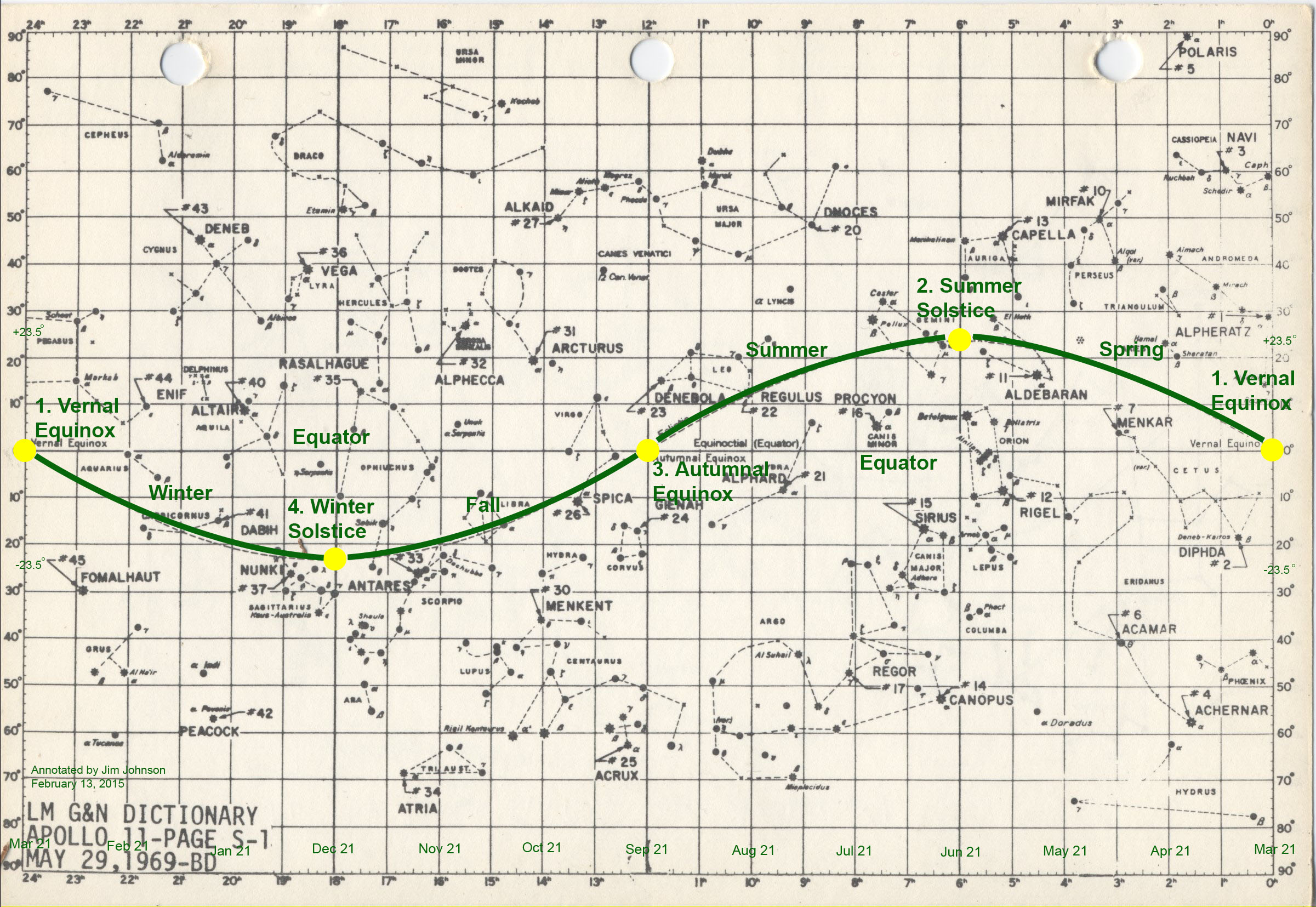
The final step in planning is to determine if Barnard’s Star’s constellation, Ophiuchus, can be viewed in the sky on the date and at the time that I wish to attempt a photograph, or 7pm in mid-October in this exercise. This step is necessary because the time of day and the time of year determines whether the desired constellation is visible in the sky, or where it is in the sky. Why? Because any object or any given set of right ascension/declination coordinates does essentially what the sun does, it makes approximately one revolution about Polaris each day due to the Earth’s rotation. Holding the time of day constant and stepping through a year’s worth of days, an object or set of coordinates makes one rotation about Polaris in a year due to the Earth’s orbit about the Sun.

To illustrate the annual rotation, lets follow Ophiuchus over the course of a year. In October it is visible in the western sky in the evening after sunset, and due to the Earth’s daily rotation about its axis, it too sets below the horizon about four hours after the sun does. Each evening, the progression of the Earth’s orbit about the sun causes Ophiuchus to appear just a little closer to the sun than it did the evening before, and the interval between sunset and Ophiuchus setting below the horizon gets almost imperceptibly shorter from one evening to the next. Two months later in December, Ophiuchus has already set below the horizon before it is dark enough to see its stars. Between December and January, the Sun is located near the star field represented by Ophiuchus, and rendering it completely impossible to see this constellation at any time during the day. By January, Ophiuchus can be seen again as it emerges from behind the sun, and rises in the east just before sunrise. Each morning, it rises just a little earlier, and by May it rises in the east just after sunset, which means that it is easily seen in the early evening. And finally, by October it is once again visible in the west as soon as it is dark enough to be seen.

To complete this final planning step, I set a planosphere for 7pm in October, and I could also see that Ophiuchus was above the horizon in the west. With an observation plan in hand, and having ascertained that the target will be well-placed in the sky, I begin monitoring my observatory’s Clear Sky Chart to find a suitable evening to set up the telescope and execute my plan.

FINDING

A clear evening finally arrives, so it is now time to begin working outdoors at the telescope. To follow along, first open and examine the wide field chart, which charts the stars that I can expect to see with my unaided eye. Since I cannot see Barnard’s Star directly, I will have to work with what I can see to help me point the telescope toward the star field where Barnard’s Star is located. First, examine the wide field chart to become familiar with the constellation and the location of Barnard’s Star therein. The red circle and rectangle near the center of the image are centered on Barnard’s Star, even though this particular star is not bright enough to appear on this chart. Note the right ascension and declination coordinates on the bottom and left edges of the chart, and that the circle and rectangle are indeed centered on the coordinates that I looked up earlier on Wikipedia. The circle represents the field of view of the Panoptic 35mm eyepiece that I intend to use to directly view the star field, and the rectangle represents the field of view of the Canon EOS 60Da camera with which I will capture images. Also note in the upper left corner of the image that stars of magnitude 5 and brighter are displayed, and that the field of view is almost 180 degrees, or essentially the whole visible sky.

With this sense of scale to help me determine where to point the telescope, I proceed by devising a star hopping strategy. I select Beta Ophiuchus as my visual jumping off point to Barnard’s Star, and since this star is not easily confirmed in my light-polluted back yard, I first locate the brightest, closest, most easily identified object that I can find, The Summer Triangle. In the chart, the Triangle stars, connected by my light colored triangle annnotation, are Alpha Lyra (Vega), Alpha Cygnus (Deneb), and Alpha Aguila (Altair). I first hop from Altair and Vega via the red lines to Alpha Ophiuchus, the brighest star in that constellation and then down to Beta Ophiuchus, the second brightest star and my jumping off point for arriving in the vicinity of Barnard’s Star. I then find all of these stars in the sky, eyeball the scale and distance, and place the telescope’s red dot finder to the point in the sky just to the left of Beta Ophiuchus.

To follow at this stage, open the medium-field of view chart and examine it. There are a few things to note here. First, the magnitude in this chart is increased to display stars down to magnitude 10.3 and brighter, there are now stars visible within the circle and rectangle, and the circle and rectangle appear much larger as the field of view has narrowed from 180 degrees down to 11 degrees. Second, I note the two most distinct objects in the chart: the sharks nose (my naming) asterism of stars that I connected with red line segments in the upper left of the rectangle, and Ophiuchus 66 in the lower left of the rectangle. If I can bring the the shark’s nose and Ophiuchus 66, which is much brighter than anything near it, into the eyepiece field of view, then Barnard’s Star (white carat) must also be in the field of view. The implication of this fact meant that I did not need to positively identify Barnard’s Star while I was a viewing at the eyepiece. I could, however, see what I thought to be Barnard’s Star, but the dimmer stars needed to confirm this sighting were not visible in the eyepiece.

It is time to locate the desired star field in the eyepiece and capture an image. The wider field of view of the eyepiece compared to the camera’s field of view, and the fact that I can see the star field move in the eyepiece in real time as I search for the correct star field helps me locate the correct star field much faster. On the night that the image was captured, I was fortunate to find the shark’s nose asterism and Ophiuchus 66 with only minor moving around once I pointed the red dot finder just to the left of Beta Ophiuchus. Next, I centered up my intermediate targets in the eyepiece, and swapped out the eyepiece for the camera at the telescope’s rear aperature and refocused. I snapped a single 25-second image, and voila, I could see the asterism and Ophiuchus 66 in the camera’s rear display. Open the actual full frame image that I captured and do a side-by-side comparison with the medium field of view chart. Also note that the orientation of the full frame image and the frame in the medium field of view chart are not the same. It was not important that the camera frame have the same orientation as the chart, because my mission in life at this point was simply to capture the shark’s nose and Ophiuchus 66 in the same frame.

ANALYSIS

I am back indoors at the computer, and not necessarily on the same night, to perform the analysis that will confirm that I found Barnard’s Star. To follow along at this stage, open the close field of view chart. Note that it display stars all the way down to magnitude 14.2, and many more stars are visible. The field of view, which is now only about 1 1/2 degrees (compared to the original 180 degree field of view), is completely inside of the camera’s rectangular field of view as noted by the rectangle in the previous chart. Ophiuchus 66 can be seen way down in the lower left corner, and I connected the shark’s nose stars with a white dotted line. In order to positively identify Barnard’s star, which is annotated, I first matched the brighter stars in the chart with those in the in the image. I used a red line in the image to mark a star hopping path from the tip of the shark’s nose through the dimmer stars down to Barnard’s Star, and I highlighted a wishbone asterism that caught my eye in some online images of Barnard’s Star. Open the cropped image of the star field and do a side-by-side comparison with the image of the close field chart, and see if you can star hop from the tip of the shark’s nose to Barnard’s Star in the cropped image. For extra credit, devise an alternate star hopping path and reconfirm the result, or even repeat this exercise in any Barnard’s Star image that you find online.

CLOSING

I feel a great sense of accomplishment in finding and photographing this star, and it pleases me greatly to share my work. I should share with you that this exercise was slightly over-simplified, because no transformation is required to equate the chart view to the images captured by the camera. At the eyepiece, a star field may be flipped horizontally, vertically or in both directions, depending upon the type of telescope (reflector or refractor) and whether a 90-degree prism is in the optical path determines whether transformation is required. If needed, the chart can be set to display the stars as they will be seen in the eyepiece by flipping the chart horizontally, vertically, or in both directions to match the eyepiece view.

So what’s next? I have known since childhood that Barnard’s Star has the fastest proper motion of any star that we can see from Earth, and I have dreamt of demonstrating this motion for myself for as long as I have known this fact. Sure, I can look at existing images of the star field that have been taken during my lifetime, and plot its motion. But now that I have captured my own baseline image, I need only capture another image at some point in the sufficiently distant future and note that its location has shifted from the baseline image, and I will have demonstrated this motion for myself! The optics/sensor combination that I used in October equates to about 1.6 arcseconds per pixel, and Barnard’s Star’s movement of 10.3 arcseconds/per year should result in about six pixels of movement relative to the background stars. I will take a second photograph in a year, and attempt to detect Barnard’s Star’s movement, and report back my finding.

An interesting consequence of Barnard’s Star being so close to us is that it has a very high parallax shift against the “fixed” background stars as the Earth moves from one side of the Sun to the other in a six-month, or half-orbit period. To demonstrate parallax shift, hold a pencil point out at arm’s length, close one eye and note the point’s position against the more distant background. Without moving the pencil, view the pencil point with the other eye open, and close the first eye. Note how the point shifts against the background. Before six months from October rolls around, I will be doing some analysis to determine if it is possible for me to detect Barnard’s parallax shift against the background stars in April when the Earth has moved around to the other side of the Sun. The distance between the two observation points, which is analogous to the distance between one’s eyes in the pencil illustration, is roughly 193-million miles. If it is mathematically possible with my telescope/sensor combination, I will attempt to detect Barnard’s parallax shift and report back.

As a bonus, this exercise has demonstrated that imaging Pluto is within my reach! The prospect of producing my own images of Pluto (still a planet in my mind, logical arguments for why Pluto is or isn’t a planet notwithstanding!) also captured my imagination in grade school when I saw first saw Clyde Tombaugh’s pair of images taken on the nights of the 23rd and 29th of January in 1931. Next July 4th, when Pluto and Earth are at their closest approach for 2015, Pluto’s angular velocity will be about 1 1/2 arcminutes per day, which is almost 200,000 times faster than Barnard’s Star’s motion (10.3 arcseconds) against the background stars! This means that I can detect Pluto’s motion by taking images just a few days apart instead a year apart. Pluto’s magnitude will be about 14.1, which is brighter than some of the stars that are visible in my Barnard’s Star image. I can improve my chances of detecting Pluto by exposing just a little longer, and by stacking multiple images to reduce background noise.

© 2014 James R. Johnson
jim@jrjohnson.net

The Speed of Light

Light travels in photons that are either emitted from hot objects like light bulb filaments, or reflected off of cooler objects, like the walls. The Sun and Moon are also emission and reflection objects, respectively. Photons travel from their source to our eye or camera sensor at, well, the speed of light. We can express this speed in terms with which we are already accustomed, like miles per hour (mph). Since light travels at 186,282 miles per second, that equates to 670.6 million mph. That is incredibly fast! Since mph has a distance component (miles), we can use the speed of light, or the speed of anything else, to measure distance. If something is 670.6 million miles away, we can also say that it is one light-hour away.

The amount of time involved essentially becomes the yardstick. The Moon is about two light-seconds away. The Sun is eight light-minutes away. A light-hour does not get us all the way to Saturn, and the closest star is four light-years away. Galactic sizes are on the scale of hundreds of thousands of light-years, and intergalactic distances are on the scale of millions and even billions of light-years. There’s nothing like the distances across the vast emptiness of space to make light seem to flow like molasses.

An implication of light’s incredibly slow speed is that our eyes are essentially time machines. The point at which Saturn appears in the sky is actually where it was over an hour ago. Similarly, The Andromeda Galaxy, our closest galactic neighbor, is seen as it was 2.5 million years ago. A supernova detected today in a galaxy located 11 million light-years away actually happened 11 million years ago.

It is entirely possible that Betelgeuse, 650 light years away, has already gone supernova, and that information has not yet reached Earth.

The Milky Way: How to See our Galaxy

The Milky Way Galaxy is the galaxy that contains our solar system. Milky Way also refers to the diffuse band of light that arcs across the summer sky from Sagittarius in the southeast to Cassiopeia in northwest. It’s name is derived from its “spilled milk” appearance.

I recall seeing the Milky Way often as a child growing up in semi-rural Georgia, but I have not been able to see it where I presently live because the light-polluted sky is brighter than the Milky Way. It is best seen as far away from city lights as possible, and on a Moonless night.

What I hope to do in my treatment of the Milky Way is relate the band of light that is seen stretched across they sky to the structure of the spiral galaxy that the Milky Way actually is. In order to make this leap, I must do three things: 1) describe a spiral galaxy’s structure and appearance by using far away galaxies and a Frisbee as proxies, 2) describe the Solar System’s location within the Milky Way Galaxy, and 3) take an imaginary journey to our location inside of the Milky Way Galaxy.

Before proceeding, it will be helpful for us to reacquaint ourselves with light and time, and their relationship to distance. Light travels in photons that are either emitted from hot objects like light bulb filaments, or reflected off of cooler objects, like the walls. The Sun and Moon are also emission and reflection objects, respectively. Photons travel from their source to our eye or camera sensor at, well, the speed of light. We can express this speed in terms with which we are already accustomed, like miles per hour (mph). Since light travels at 186,282 miles per second, that equates to 670.6 million mph. That is incredibly fast! Since mph has a distance component (miles), we can use the speed of light, or the speed of anything else, to measure distance. If something is 670.6 million miles away, we can also say that it is one light-hour away.

The amount of time involved essentially becomes the yardstick. The Moon is about two light-seconds away. The Sun is eight light-minutes away. A light-hour does not get us all the way to Saturn, and the closest star is four light-years away. Galactic sizes are on the scale of hundreds of thousands of light-years, and intergalactic distances are on the scale of millions and even billions of light-years. There’s nothing like the distances across the vast emptiness of space to make light seem to flow like molasses.

An implication of light’s incredibly slow speed is that our eyes are essentially time machines. The point at which Saturn appears in the sky is actually where it was over an hour ago. Similarly, The Andromeda Galaxy, our closest galactic neighbor, is seen as it was 2.5 million years ago. A supernova detected today in a galaxy located 11 million light-years away actually happened 11 million years ago. With your mind sufficiently bent, let’s proceed on our three-step journey to “see” our place in the galaxy.

1. Structure and Appearance of a Spiral Galaxy
We can learn much about the structure of a spiral galaxy by observing neighboring galaxies that we can see from various perspectives. We learn from these observations that a typical spiral galaxy is a disk that is thin at its edges, and becomes thicker at points toward the center. There are essentially three perspectives that matter: face-on, edge-on, and in any perspective between the two.

The first perspective to consider is that of a galaxy viewed edge-on. From this perspective, a galaxy’s profile is thin at its edges and it grows increasingly thicker toward the center, and there is a noticeable bulge at the galaxy’s center. The line of sight is through the longest dimension of the disk, so billions of stars contribute to a distant galaxy’s faint glow that we perceive through an amateur telescope. These features can be seen in NGC 4565, which is an example of an edge-on galaxy located about 43 million light-years away. Zoom in on the image at the link and notice that there are brighter areas were masses of stars can be seen, and other areas where the stars are obscured by dust lanes. A Frisbee flying toward you at eye level would present a profile similar to that of an edge-on galaxy.

The second perspective to consider is that of a galaxy viewed face-on. It will appear as a near perfect circle with spiral arms of dust and stars. Generally, a face-on galaxy will be brighter in its center, because stars are more densely aggregated about the galactic center, and because the disk is thickest at the center bulge. Messier M74, located about 32 million light-years away, is an example of a galaxy viewed face-on. Click on the image and zoom in, and again notice the bands of stars and bands of dust. A Frisbee seen lying on the ground has a similar circular profile.

A third perspective would be a view from any perspective other than edge-on or face-on. The profile of such a galaxy is elliptical, with the flatness of the ellipse being related to the offset angle. Messier M31 (Andromeda Galaxy) is an example that is located 2.5 million light-years away, which makes it the Milky Way’s closest galactic neighbor. Our Earth-bound view of M31 is about half way between edge-on and face-on perspectives. Zoom in on the image at the link to see all of the features previously described in the face-on and edge-on perspectives of galaxies.

Even though a galaxy contains billions of stars, it is important to keep in mind that a galaxy is mostly vast tracts of empty space. Our galaxy is so vast in size that we can only see a tiny bit of it. It is believed to be about 120,000 light-years in diameter and it is believed to contain about 250 billion stars. In contrast, the farthest star that we can see with the unaided eye is a very bright one that is about 4,000 light-years away, but something on the order of 500 light-years is typical of the most distant stars that we can easily see from Earth. Within this radius, that are only about 5,000 individually resolvable stars that can be seen by the unaided eye. When stars are viewed at greater distances, they are too dim to resolve individually and the apparent distance between stars grows smaller. As a result, when looking toward the center of our galaxy where stars are more densely packed, we see literally billions of stars that are too dim to be individually resolved, but the combined effect of these billions of stars is that they are perceived as a diffuse patches of light.

2. Location of the Solar System.
The solar system is located within the flat disk of the Milky Way Galaxy, and is about 27,000 light-years from its center. Since The Milky Way Galaxy’s diameter is 120,000 light-years, its radius is 60,000 light years. Thus, we are located just inside a point about half way between the center of the galaxy and its outer edge. Since there are more stars concentrated in the galaxy’s center we will see more stars when gazing in that direction than when we are gazing outward toward the nearest edge where stars are more sparsely spread. To mark a corollary of our location on say a 10″ Frisbee, one could put a star sticker about 4 1/2 inches from its center. More precisely, our location is beneath the star, somewhere about half way between the top and bottom of the Frisbee’s cross section.

3. A Journey to the Solar System
Let’s begin our imaginary journey to the Solar System’s location within the Milky Way Galaxy. In order to scale this journey down to something we can more easily understand, we will once again employ the Frisbee proxy. To orient ourselves, lets first stand near the Frisbee and look down upon it observing a profile similar to the face-on view of the galaxy. Note the location of the star sticker that we put on the Frisbee to mark our notional location. Now place yourself at a point where you are on a line drawn outward from the center of the Frisbee through the star sticker, and now take three or four steps away from the Frisbee in the direction of this line, and place your eyes down at ground level so that the Frisbee is viewed edge-on, and imagine that the Frisbee is our own Milky Way Galaxy. Initially, the view of the galaxy will appear similar to the example edge-on galaxy, NGC 4565, that we examined earlier. Please have this image fresh in your mind before we start moving, because this is how our galaxy appears from our initial vantage point.

At long last we begin our journey, and as we approach the Milky Way Galaxy, its appearance does not change much from the edge on view of NGC 4565. It will only grow proportionately wider and thicker in size as we move closer to the Milky Way’s center. At about 300 light-years from the disk’s edge, individual stars immediately ahead become individually resolvable. A glance in the direction away from the Milky Way is eerily devoid of stars . Once inside the edge, the nearest stars will begin to “fly” past us in a manner similar to what is seen on certain Windows screen savers or on Star Trek. Ahead of us we still see the patchy fog of the dense galactic core as the backdrop for the foreground stars, and behind us we can see some stars, but against a completely dark backdrop. Finally, we reach the Solar System and stop. Because an overwhelming majority of all the Milky Way’s stars are still ahead of us in its dense center, the only significant change in the galaxy’s appearance since we began our journey is that it grew wider and thicker as we moved closer.

Now that we understand a spiral galaxy’s structure and appearance, know our location in the Milky Way Galaxy, and have seen what happens as we fly into the galaxy from its edge, let’s now examine a fish eye photographic image of the Milky Way on the National Geographic Web site. The Milky Way appears as an arch in this image due to fisheye distortion, so to get a true perspective, imagine that the arch is straightened out. Compare this Milky Way image with the edge-on image of NGC 4565 previously viewed. Can you see…bright patches of unresolved stars? …dark dust lanes? …a flattened, edge-on disk? …a bright central bulge? Armed with enough information, it is possible to gaze upon the Milky Way as seen in the summer sky from Earth and understand that it is actually the disk of the Milky Way Galaxy!

© James R. Johnson, 2014.
jim@jrjohnson.net

The Inclination of Saturn’s Rings

As Saturn cycles through its 29 1/2 year orbit about the Sun, we on Earth will alternatively see the top (north face) of Saturn’s rings for roughly half of its orbit, and the bottom half (south face) of Saturn’s rings for the other half. This occurs as a result of how the rings are inclined with respect to the plane of Saturn’s orbit. As the view transitions between upper and lower halves of the rings, our view will be edge on, and the rings will seem to have temporarily vanished. The last edge-on view was in 2009, at which time our current view of the north face of the rings began opening up. Even before Saturn’s rings fully open in 2017, our present view is pretty spectacular.

Collimating a Schmidt-Cassegrain Telescope

Telescope collimation refers to alignment of the elements in its optical system. Perfect alignment is required to achieve optimal performance of any optical system. Otherwise, contrast and detail are lost. This guide focuses (pun intended) on the Schmidt-Cassegrain Telescope (SCT) design, which is susceptible to misalignment. Periodic collimation is required for casual observing to correct misalignment that results from normal handling and transportation of the telescope. Even more frequent collimation is required of the perfectionist who wishes to account for collimation errors caused by pointing the SCT at different objects at different positions. This is what can occur when a telescope “leans” in another direction after collimation has been perfected. When seeking high resolution at higher magnifications, one should ideally collimate on every object observed or photographed. This might seem like an excessive burden, but it becomes second nature and can be quickly accomplished with practice. The superior result produced by perfect collimation is worth this price.

Few people, other than astronomers, appreciate the multiple skill sets that are required to plan, set up, and execute an observing or imaging session. Collimation is just another skill that an astronomer must master, because the difference between mediocre and great collimation is astounding! I cannot imagine why an astronomer would put so much effort into a session without checking collimation, and adjusting if necessary. My goal in writing this article is to shorten the learning curve to achieving really good collimation with the hope that astronomers will be more inclined to adopt collimation as a regular part of their set up.

This guide begins with a description of the phenomenology that is evaluated to determine if precise collimation is achieved. Next is a description of an SCT optical system, and how it is adjusted to achieve precise collimation. After the phenomenology involved and the SCT optical system are understood, the basics of collimating an SCT can be explored along with the rational that explains the details behind each concept. With a firm grasp of the basics, all that is left is to provide the procedures that are used to actually collimate an SCT.

The Phenomenology

A collimation process can be followed with great results without really understanding the telescope or the phenomenology that is being exloited, but that is seldom satisfactory for astronomers. They often want a deeper understanding of what is really going on in order to permit application of expert judgement in their tradecraft. In order to understand what is really going on, an explanation of some phenomena and concepts is required. The key phenomena associated with collimation is the concept of a pinpoint light source, and how it interacts with an optical system. In addition to collimation and a pinpoint light source, I will also cover the Airy disk and diffraction rings.

The essence of collimation is how photons travel with respect to one another. Light from a point source arriving at an optical system is considered collimated if all photons are travelling parallel to one another. A collimated optical system transmits collimated light to a single point at the focal plane. Generating a collimated light source for a microscope might be tricky, but Astronomers are lucky. They have access to a sky full of collimated pinpoint light sources. Each star is so far away that it cannot be magnified larger than a single point, and thus all of the photons arriving at the telescope are collimated. Consider an object like Jupiter than can be resolved to a disk with a telescope. Details on the disk can be observed because every point on the disk is a separate pinpoint light source. A telescope’s job is to preserve all of these pinpoint sources through the optical path to the focal plane. A telescope can only achieve this feat when correctly collimated.

The Airy disk is named after George Biddell Airy, who in 1835 provided the first theoretical description of how an optical system resolves a pinpoint light source. The Airy disk is the smallest disk that is formed by a pinpoint light source in a given optical system. All other things being equal in two telescopes, the telescope with the larger aperture is said to have more resolving power, because it is capable of resolving a pinpoint light source into a smaller Airy disk. This smallest disk implies perfect focus, and any other focus position produces an enlarged blob of light. Surrounding the Airy disk is one or more alternating light and dark rings of equal spacing known as diffraction rings. These rings can be seen only under the very best seeing conditions. Diffraction rings are formed as the result of light waves interacting with the circular aperture of the telescope. The spacing of these rings is a function of wavelength of the light.

The SCT Optical System

The optical path of an SCT from entry to exit consists of a corrector plate, a primary mirror, and a secondary mirror. For this discussion, front means the end of the telescope pointing toward the observed object, and back means the other end of the telescope where the gathered light is focused onto an eyepiece or sensor. Light arriving at an SCT first encounters the corrector plate at the front of the telescope. The corrector plate is so gently curved that it has the appearance of a flat pane of glass. The purpose of its optical curvature is to correct for spherical aberration. This is necessary because the next optical component, the primary mirror, is spherically curved, which means that it is incapable of bringing light rays to a single point of focus without a corrector. The aperture of an SCT is determined by the diameter of the primary mirror, which is located at the back of the telescope. It reflects light forward toward a focal point. This mirror is perforated at its center, and it can be adjusted forward or backward to achieve focus. The next element in the optical path is the secondary mirror, which is mounted in the center of the corrector plate. It is usually spherical in shape, which continues to focus the light. This is the final optical component that the light encounters before achieving focus just to the rear of the center perforation in the primary mirror.

The Basics

This guide offers a couple of techniques rough collimation techniques should be used before proceeding to the precision collimation procedure, unless a precise collimation was obtained during a recent observing session. Before proceeding to the details of either a rough or precise collimation, There are some basics that apply to all collimation techniques. Do not attempt to follow these basic steps, but do read them carefully to understand the concepts before proceeding to and actually following the rough or precise alignment procedures. Before collimating, always allow the telescope to thermally stabilize, which could take an hour or more.

Tilting the secondary mirror with respect to the primary mirror is the only mechanical adjustment required to collimate an SCT. Looking at the front of the telescope, the secondary mirror housing is located in the center of the corrector plate. If a central screw is present on the front of this housing, it should never be adjusted. Somewhere between the center of the housing and its outside edge are three adjustment screws situated 120° apart. The mirror itself is located on the back side of this housing. The adjustment screws control the tilt of the secondary mirror, and they hold it in tension against a central pivot. The tilt of the mirror is changed by loosening and tightening the adjustment screws, thereby pivoting the mirror about the central pivot. A single adjustment requires that all three screws be turned in order to change the tilt AND maintain the tension. For instance, if a certain adjustment screw must be tightened to achieve a desired effect, then the other two screws must first be loosened to prevent the adjustment without over tightening the first screw. Conversely, if a screw must be loosened, then loosen that screw first and complete the adjustment by tightening the other two screws to keep the mirror snug against the central pivot. Most SCTs come with adjustment screws, but after market adjustment knobs that are easier to use are available. That knobs can effectively hold collimation is the subject of debate. I recommend screws if collimation is only checked periodically to ensure that collimation remains acceptable over a longer period of time. Knobs, being easier to adjust, are probably just fine when collimation is checked frequently. Did I say that the central screw, if present, should never be adjusted?

A defocused pinpoint light source is used for rough collimation, and in the initial step of a precise collimation. When defocusing a pinpoint light source, three things become apparent. First the pinpoint becomes a diffuse blob. All of the same photons are still there, they are just spread over a larger area. It becomes easier to detect a collimation error the more the telescope is defocused. Next, notice that the center of the blob will blacked out. This is the shadow of the secondary mirror. And lastly, defraction circles will surround the central black blob. The central shadow and the defraction rings viewed in a perfectly collimated telescope will appear perfectly round, and perfectly centered within one another. Anything else is an uncollimated telescope, and adjustment is required to achieve perfect collimation.

In order to adjust collimation, the adjustment screws or knobs are turned in small increments. The result is then checked at the eyepiece. If the adjustment improves collimation, continue to make small adjustments in that direction until achieving perfection. If collimation worsens, adjust back to the original position, and make a small adjustment in the opposite direction. The adjustment screws should be snug, not tight or loose. If a screws should seem overly tight or loose while adjusting, slightly adjust the other two screws in the opposite direction.

Short arms vs. long telescope. If the person doing the collimation has long arms and a short telescope, it may be possible to turn the adjustment screws while observing the effect in the eye piece in real time. More often, this is not the case. Two people working together might be effective, especially if these two people work together often, and know how to collimate with minimal communication. Usually, an experienced collimator will be able to get the job done quickly working alone. As a guide to determine which screw to adjust, a person working alone can observe the direction in which collimation is off, and determine which screw to adjust by putting a finger or other thin object in front of the objective in that direction. Once the finger and the collimation error are aligned, it will be pointing to the screw that requires adjustment.

Some steps will require that the telescope be purposefully defocused. The out of focus position can be either inside of focus, or outside of focus. It really does not make any difference technically. A habit of always defocusing in the same direction simplifies the collimation process by making the results of a given action predictable. This permits one to quickly develop a sense of which adjustment screw to turn, and in which direction it should be turned.

Whether or not to collimate with a star diagonal in the optics path is another point of debate. A high-quality diagonal in the optics path is acceptable if this configuration is contemplated for visual observation. Keep in mind that the directional effects of a certain adjustment to which one has become accustomed my be reversed. There is no good reason to place a diagonal in the optical path for astrophotography, so remove the diagonal when collimating for astrophotography. So finally, here are the basic collimation steps:

  1. Thermally stabilize the telescope
  2. Center the collimation target in the eyepiece
  3. Adjust the collimation screws to achieve the desired result
  4. Re-center the collimation target in the eyepiece
  5. Repeat until there is no need to re-center in the eyepiece

When collimating for absolute perfection, the best collimation target is always a star near the object to be observed in a dark sky under good seeing conditions. For a more casual collimation, there are some alternative targets that can be used for periodic or rough collimation. A star is still the best point source of light, and a dark sky with good seeing conditions is still desired. For even better seeing, select a star near the zenith.

Any alternative target must simulate the pinpoint light source that a star presents, and it must be placed sufficiently distant from the telescope that the telescope can be focused. Commercially manufactured laser targets are probably slightly better than the others that will be mentioned here. Because of the added cost and the added calibration steps of a laser target, and how easily an SCT might loose perfect collimation, this is not be an attractive alternative for collimating an SCT. Other alternative targets are deceptively simple. I have never used it, but the idea that I like is a chrome ball bearing in direct sunlight. There is only one pinpoint spot on the ball bearing that reflects sunlight back toward the telescope. A glass Christmas tree ball works as well. Another is a bulb in a box, with the open end facing the telescope, and covered with a pin-pricked sheet of aluminum foil.

That covers the basics, so now on to the actual collimation procedure. I divide the procedures into rough and precise. In the precise procedure, I further call out what is needed for the occasional collimation or for even more precise collimation that would be conducted before every observation or image capture.

Collimation Procedures

Rough Collimation.

  1. Select an eyepiece that provides a magnification of roughly the aperture of the telescope in millimeters. E.g., an 11″ telescope aperture is 280mm, so use an eyepiece that provides about 280x magnification. For an 11″ F/10 telescope, which has a 2800mm focal length, use a 10mm eyepiece (magnification = telescope focal length/eyepiece focal length)
  2. Select a bright target star of 1st magnitude or greater, or use one of the alternative targets previously described
  3. Defocus as much as possible to reveal the collimation error, if any. Proceed to Precise Collimation if no error can be detected.
  4. Determine which screw will correct the error, and adjust 1/8 turn in the required direction
  5. Return to the eye piece, recenter the target, and readjust if necessary
  6. Repeat the last two steps until recentering and readjusting is no longer necessary

Precise Collimation.

  1. Select an eye piece magnifies 2x the telescope aperature in millimeters. Using the 11″ telescope example, 560x, which would require at least 5mm focal length eye piece
  2. Select a target star of 2nd (e.g. Polaris) or 3rd magnitude near the zenith for casual/infrequent collimation, or near the object to be observed for a one-time collimation
  3. Defocus as much as possible to reveal the collimation error, if any
  4. Determine which screw will correct the error, adjust 1/8 turn in the required direction
  5. Return to the eye piece, recenter the target, readjust if necessary. Proceed to Step 7 if no error is detected.
  6. Repeat the last two steps until recentering and readjusting is no longer necessary
  7. Precisely focus the star, and observe first diffraction ring in the airy disk pattern. Note, the airy disk will not be visible under marginal seeing conditions.
  8. Adjust, if necessary, using 1/16th turn at a time until the first diffraction ring around the disk is complete and uniform

Conclusion

This completes our examination of SCT collimation for casual visual observation or precise astrophotography. First, we explored the phenomenology that make collimation possible, and the SCT optical system that is of interest to us. Following next was the the a detailed treatment basics of collimating an SCT, along with the rational that explained the details behind each concept. Lastly, detailed procedures were provided to guide a knowledgeable astronomer through rough and precision collimation of an SCT. I frequently refesh my memory be reading through the entire article, and to make sure that I do not miss anything, I actually open and use these procedures when I collimate. You are welcome to do the same, and your feedback and suggestions will be valued.

© James R. Johnson, 2014.